Spectral Signatures of Sector Bubbles: AI Era vs Dot-Com

Quantitative exploratory analysis. Data covers January 1997 – December 2002 and January 2023 – October 2026.

Disclaimer: This analysis is for research and educational purposes only and does not constitute investment advice.

1. Abstract

I test whether the current AI sector exhibits the correlation structure signatures observed during the dot-com bubble (1997-2002). Using spectral analysis of rolling correlation matrices on Fama-French 49 industry portfolios (following Buccheri, Marmi & Mantegna (2013)) I compare three diagnostics metrics across both eras: dominant eigenvalue evolution (λ₁), intra-sector vs cross-sector correlation gap ( herding), and second-mode eigenvector loadings (λ₂ decoupling). I found that while AI-adjacent industries show elevated within-group correlation, the defining spectral signature of the dot-com bubble (a clear tech vs rest decoupling in λ₂) is absent in this actual era. The results suggest the current AI enthusiasm, as of late 2026, does not replicate the correlation regime that preceded the dot-com crash.

2. Introduction & Motivation

The rapid ascent of artificial intelligence stocks since 2023 has drawn frequent comparison to the dot-com bubble of the late 1990s. NVIDIA’s capitalization surpassed $5 trillion, AI-adjacent companies saw triple-digit returns, and a handful of technology names began dominating index performance. The parallel is tempting, and widely repeated in financial media.

But is it accurate? Popular comparisons typically rely on price charts and valuation multiples. Most of the time, these are just noisy, context-dependent, and easy to cherry-pick. A more structural question is whether the correlation regime of today’s market resembles the one that preceded the dot-com crash.

During a sector bubble, a distinctive pattern emerges in the correlation structure of asset returns. The bubble sector begins to move as a tightly correlated block, herding, while simultaneously decoupling from the rest of the market. This creates a measurable spectral signature: the second eigenvalue (λ₂) of the rolling correlation matrix spikes, and its associated eigenvector splits cleanly into the bubble sector versus everything else. Buccheri, Marmi & Mantegna (2013) documented this pattern in the dot-com era using spectral decomposition of correlation matrices.

In this study, I apply the same methodology to both periods. Using Fama-French 49 industry portfolios, I compute rolling correlation matrices and track the diagnostic metrics across the dot-com era (1997-2002) and the AI era (2023-2026): dominant eigenvalues share (λ₁), intra-sector versus cross sector correlation gap, and second mode eigenvector loadings.

If the AI boom is structurally similar to the dot-com bubble, these metrics should show comparable signatures.

3. Data

I use the Fama-French 49 industry portfolios, obtained from Kenneth French’s data library. These portfolios aggregate all CRSP-listed stocks into 49 industry groups based on SIC codes, providing daily value-weighted returns. The dataset is widely used in empirical finance research for two reasons: it is survivorship bias free (delisted firms remain in the historical record), and its industry classification is consistent across decades, enabling direct cross-era comparison.

I analyze two periods:

• Dot-com era: January 1997- December 2002, capturing the full bubble formation, peak and crash.
• AI era: January 2023 - October 2026, capturing the current AI-driven market regime.

Both periods use the same 49-industry structure, ensuring an apples-to-apples comparison. An earlier version to this analysis used individual AI adjacent stocks (NVDA, MSFT, META, etc.) for the AI era, but the difference in data granularity introduced systematic noise differences that complicated interpretation. I retain the individual stock analysis as a supplementary exercise but base all cross-era conclusions on the Fama-French data.

All returns are converted from percentages to decimals. No additional filtering or cleaning is applied.

4. Methodology

Rolling Correlation Matrices

For each period, I compute rolling Pearson correlation matrices over a 60-trading-day window (approximately 3 calendar months). At each time step t, the correlation matrix is constructed from the returns of all 49 industries over the window [t−60, t]. This produces a time series of 49×49 symmetric positive-definite matrices.

Spectral Decomposition

Each correlation matrix is decomposed into its eigenvalues and eigenvectors using scipy.linalg.eigh, optimized for symmetric matrices. Eigenvalues are sorted in descending order. The key quantities:

• λ₁ (first eigenvalue): Measures the fraction of total variance explained by the dominant co-movement factor, “how much is the whole market moving together.” Expressed as λ₁/N × 100, where N=49.
• λ₂ (second eigenvalue): Captures the strongest residual pattern after removing the market mode. A spike in λ₂ indicates a secondary structure, typically one group of industries diverging from another.
• Eigenvector loadings of λ₂: The 49 components of the second eigenvector reveal which industries are pulling apart. Positive and negative loadings identify the two opposing groups.

Diagnostic Metrics

I track three metrics across both eras:

1. Eigenvalue evolution: λ₁/N and λ₂/N as percentages over time, measuring market-wide co-movement and sector decoupling strength.
2. Herding gap: The difference between average intra-tech correlation and average tech-vs-non-tech correlation, computed at each rolling window. Tech industries are defined as: Softw, Hardw, Chips, Telcm, BusSv, and LabEq. A rising gap indicates the tech sector moving together while pulling away from the broader market.
3. λ₂ eigenvector loadings: Examined at the peak λ₂ date for each era to identify which industries drive the decoupling mode.

Window Validation

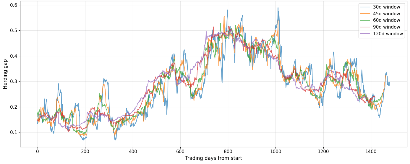
To confirm that results are not an artifact of the 60-day window choice, I repeat the herding gap analysis with windows of 30, 45, 60, 90, and 120 trading days. Results are qualitatively stable across all window sizes.

Cross-Era Comparison

Because the two periods differ in length, time-series comparisons are plotted against trading days from the start of each period rather than calendar dates. Where direct overlay is needed, metrics are z-score normalized to account for differences in scale.

5. Results

Eigenvalue Evolution

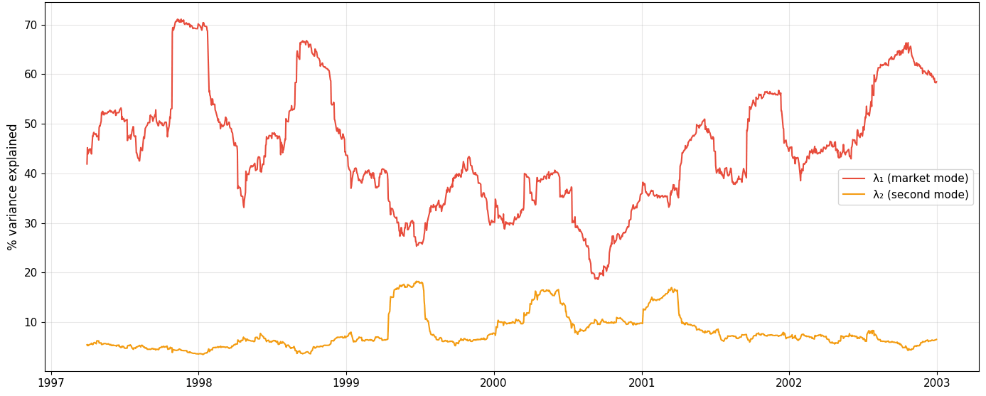
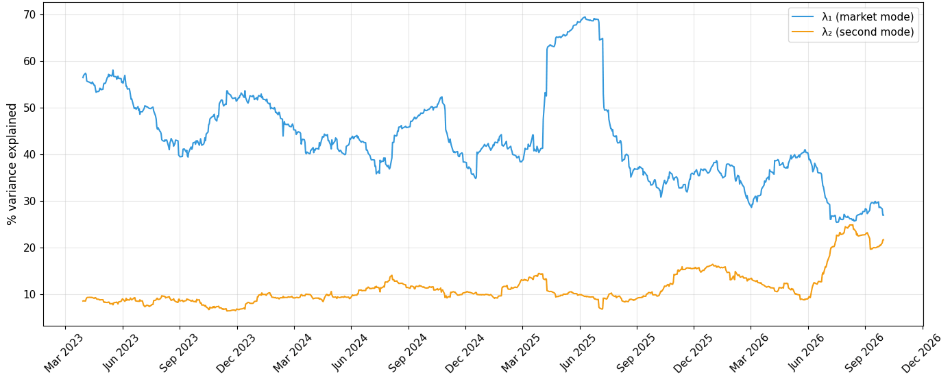
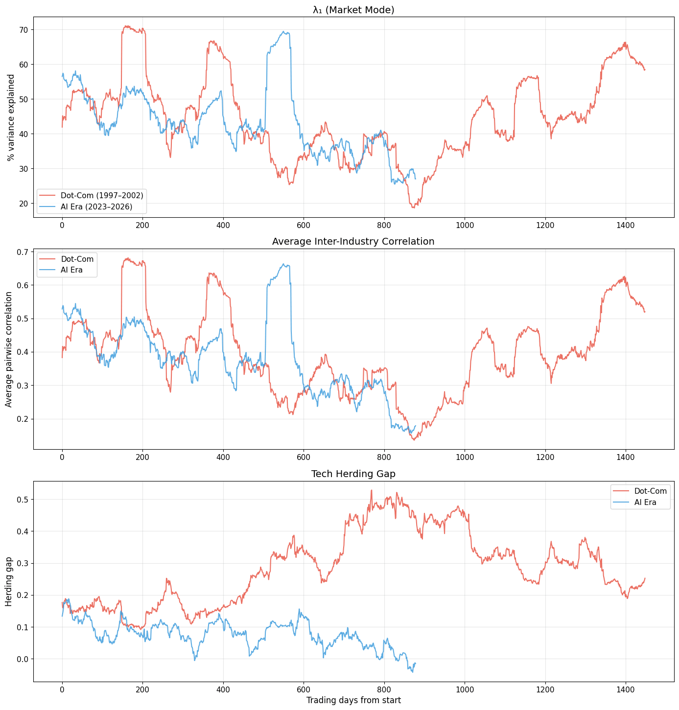
During the dot-com period, λ₁ explains 25 - 40% of total variance, rising sharply during the 2001 - 2002 crash as correlations spike market-wide. λ₂ shows distinct peaks around mid-1999 and late 2001, indicating strong secondary structure. In the AI era, λ₁ follows a similar range but without the dramatic surge. λ₂ remains lower and flatter.

Herding Gap

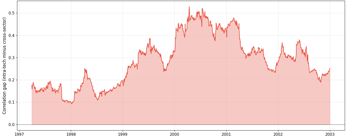
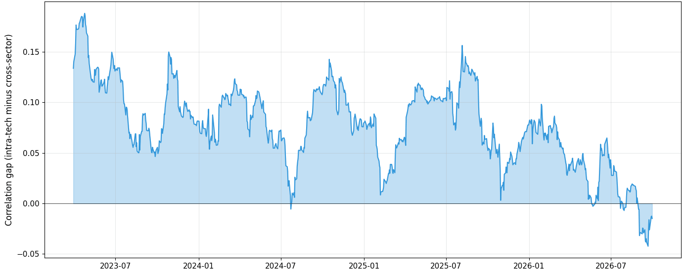
The dot-com gap rises steadily from ~0.15 in early 1997 to ~0.45 by 2000 — tech stocks increasingly moved as a correlated block while detaching from the broader market. The AI era gap shows no comparable trajectory.

λ₂ Eigenvector Loadings

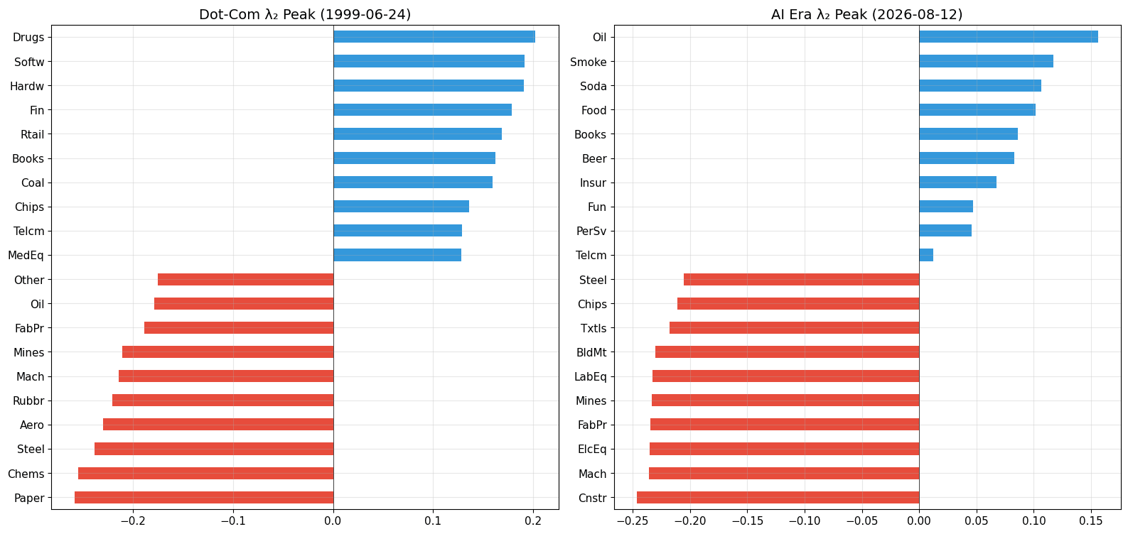
This is the most discriminating diagnostic. At the dot-com peak (mid-1999), the eigenvector splits cleanly into tech (Softw, Hardw, Chips, Telcm) versus old-economy industrials (Paper, Chems, Steel, Aero). At the AI era peak, no such split appears, the second mode separates defensive/commodity sectors (Oil, Smoke, Soda) from cyclicals (Construction, Machinery, Electrical Equipment). The AI-adjacent industries do not dominate either side.

Cross-Era Overlay

Window Validation

6. Discussion

The central finding of this study is negative: the AI era does not reproduce the correlation regime that characterized the dot-com bubble. While the popular narrative frames AI as “dot-com 2.0,” the spectral structure of the market tells a different story across all three diagnostics.

During the dot-com period, the market exhibited a textbook bubble signature, tech industries herded into a tightly correlated block (herding gap rising from 0.15 to 0.45), while the second eigenvalue spiked and its eigenvector split cleanly along tech-vs-old-economy lines. This pattern was sustained over nearly three years before the crash, building steadily rather than appearing as a brief fluctuation.

The AI era shows none of this. The herding gap remains flat and low (0.05–0.15), with no upward trend. The λ₂ eigenvector, even at its peak, separates defensive sectors from cyclicals, not tech from the rest. And in the most recent months, the herding gap turns negative, suggesting that tech industries are losing coherence as a correlated block.

Why might this be? Several structural differences between the two eras could explain the divergence:

First, AI adoption is cross-sectoral. The dot-com boom was concentrated in a narrow set of technology and telecom firms. AI, by contrast, is being adopted across healthcare, finance, energy, and manufacturing. This diffuses the “tech” signal across the entire market rather than concentrating it in one block, which is consistent with the absence of a clean tech-vs-rest eigenvector split.

Second, market structure has evolved. The proliferation of ETFs, algorithmic trading, and passive investment has changed how correlations behave. The market mode (λ₁) is structurally higher today than in the late 1990s, which may compress the space available for sector-level decoupling signals in λ₂.

Finally, The rising λ₂ in late 2026 deserves attention. While its magnitude approaches levels seen in the dot-com period, the eigenvector structure reveals a defensive-vs-cyclical rotation, likely driven by macroeconomic uncertainty (rate expectations, recession concerns) rather than tech-specific speculation. This highlights an important methodological point: eigenvalue magnitude alone is insufficient to diagnose a bubble. The eigenvector structure is what distinguishes a sector bubble from a macro-driven regime shift.

An important question this analysis cannot answer is whether AI valuations are fundamentally justified. My method detects correlation herding, not mispricing. The absence of a dot-com-style correlation regime does not mean AI stocks are fairly valued, it means the market is not treating them as a speculative bloc the way it treated internet stocks in 1998–2000. Whether the current AI investment cycle generates adequate returns remains an open empirical question for future work.

7. Limitations

This study has several limitations that should inform interpretation of the results.

Industry-level granularity. The Fama-French 49 industry portfolios aggregate individual firms into broad categories. A bubble concentrated in a handful of mega-cap names (NVIDIA, Microsoft, Meta) could be masked if the rest of their industry behaves normally. Individual-stock-level spectral analysis would provide finer resolution, though at the cost of a much larger and noisier correlation matrix.

Single methodology. I rely exclusively on eigenvalue decomposition of rolling correlation matrices. Other approaches such as log-periodic power law models, measures of trading volume synchronization, or sentiment-based indicators might detect bubble dynamics that correlation structure misses.

Window sensitivity. Although I validated results across multiple window sizes (30, 45, 60, 90, 120 days), the rolling window approach inherently smooths sharp transitions. A regime change occurring over a few trading days could be diluted within a 60-day window.

Survivorship in the AI era. While the Fama-French portfolios mitigate survivorship bias for the dot-com period, the AI era is still unfolding. If a correction occurs in the future, the current dataset captures only the buildup phase.

Correlation is not valuation. This method detects co-movement patterns, not mispricing. The dot-com bubble involved both extreme herding and extreme overvaluation. The absence of herding does not rule out overvaluation driven by other mechanisms. Conversely, the profitability of AI infrastructure companies (versus the deep losses of AI model companies) presents a more complex valuation picture than the dot-com era .

Stationarity assumption. Rolling correlation implicitly assumes local stationarity within each window. In periods of market stress, correlations can shift abruptly, violating this assumption and potentially distorting the eigenvalue decomposition.

8. Conclusion

I applied spectral analysis of rolling correlation matrices to compare the market’s correlation structure during the dot-com bubble (1997–2002) with the current AI era (2023–2026), using the Fama-French 49 industry portfolios to ensure a consistent, survivorship-bias-free comparison across both periods.

The dot-com bubble produced a clear and sustained spectral signature: the second eigenvalue rose steadily, its eigenvector split along tech-vs-non-tech lines, and the herding gap climbed from 0.15 to 0.45 over nearly three years before the crash. The AI era reproduces none of these patterns. The herding gap remains flat, the λ₂ eigenvector reflects macro-driven sector rotations rather than tech decoupling, and the most recent data shows the herding gap turning negative, implicating tech industries losing coherence as a group.

These results do not settle whether AI stocks are overvalued. They do establish that the market is not treating AI as a speculative bloc in the way it treated internet stocks in 1998–2000. A future correction in AI valuations need not reproduce the correlation pathway of the dot-com crash.

Future work could extend this analysis in several directions: applying the same framework at the individual-stock level to detect concentration within industries, incorporating alternative bubble detection methods alongside spectral analysis, and revisiting this dataset as the AI investment cycle matures, particularly to test whether the negative herding gap persists or reverses.

9. References

1. Buccheri, G., Marmi, S., & Mantegna, R. N. (2013). Evolution of correlation structure of industrial indices of US equity markets. Physical Review E, 88, 012806. DOI: 10.1103/PhysRevE.88.012806
2. Fama, E. F., & French, K. R. (1997). Industry costs of equity. Journal of Financial Economics, 43(2), 153–193.
3. Laloux, L., Cizeau, P., Bouchaud, J.-P., & Potters, M. (1999). Noise dressing of financial correlation matrices. Physical Review Letters, 83, 1467–1470.